Second Order Linear Equations, General Theory

1. Standard Form

A second order linear differential equation is a differential equation of the form

(Here A,B,C and D are certain prescribed functions of x.)

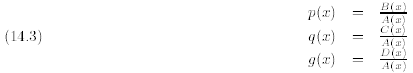
As in the case of first order linear equations, in any interval where A(x) ≠ 0, we can replace such an equation
by an equivalent one in standard form:

where

2. Homogeneous vs. Non-homogeneous Linear Differential Equations

In the development that follows it will be important to distinguish between the case when the right hand
side of

is zero or non-zero. We shall say that a second order linear ODE is homogeneous if it can be written in
the form

otherwise (if g(x) ≠ 0) we shall say that it is non-homogeneous. Note that this terminology is completely
unrelated to homogeneous equations of degree zero (the topic of the preceding lecture).

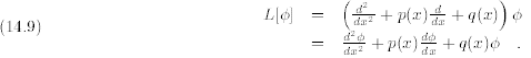
3. Differential Operator Notation

Consider the general second order linear differential equation

We shall often write differential equations like this as

where L is the linear differential operator

That is to say, L is the operator that acts on a function Ø by

4. General Theorems

The following theorem tells us the conditions for the existence and uniqueness of solutions of a second order
linear differential equation.

Theorem 14.1. If the functions p, q and g are continuous on an open interval I R containing the point
, then in some interval about there exists a unique solution to the differential equation

satisfying the prescribed initial conditions

Note how this theorem is analogous to the corresponding theorem for first order linear ODE's. Note also
that the conditions for existence and uniqueness are fairly lax - all we require is the continuity of the
functions p, q, and g around a given initial point. Finally, we note that the form of the initial conditions
involves the specification of both y(x) and its derivative y'(x) at an initial point
.
I should also point out that the preceding theorem does not address the issue of how to construct a solution
of a second order linear ODE. Indeed, the actual construction of solutions to second order linear ODE is
sufficiently complicated to that we shall spend 90% of the remaining lectures on techniques of solution. The
next two theorems at least tell us the basic ingredients for a general solution of a second order linear ODE.

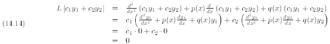
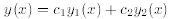
Theorem 14.2. (The Superposition Principle) If y = (x) and y = (x) are two solutions of the differential
equation

then any linear combination

of (x) and (x), where and are constants, is also a solution of (14.12).

Proof.

The fact that a linear combination of solutions of a linear, homogeneous differential equation is
also a solution is extremely important. The theory of linear homogeneous equations, including differential
equations involving higher derivatives depends strongly on the superposition principle

Example 14.3.

and

are both solutions of

It is easy to check that any linear combination of and is also a solution.

Example 14.4.

and

are both solutions of

However, it is easy to check that is not a solution of (14.20). The reason for this lies in
the fact that (14.20) is not linear.

Given two solutions and of a second order linear homogeneous differential equation

we can construct an infinite number of other solutions

by letting and run through R. The following question then arises: are all the solutions of (14.21)
capable of being expressed in form (14.22) for some choice of and ?

This will not always be the case; and so we shall say that two solutions and form a fundamental set
of solutions to (14.21) if every solution of (14.21) can be expressed as a linear combination of and
.
Theorem 14.5. If p and q are continuous on an open interval I = ( α, β) and if and are solutions of
the differential equation

satisfying

at every point x∈ I, then any other solution of (14.23) on the interval I can be expressed uniquely as a
linear combination of and .

Proof.

Let and be two given solutions on an interval I and let Y be an any other solution on I. Choose a
point ∈I. From our basic uniqueness and existence theorem (Theorem 3.2), we know that there is only
solution y(x) of (14.23) such that

namely, Y (x). Therefore if we can show that a solution of the form

satisfies the initial conditions (14.25), then we must have 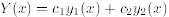and so Y (x) is a linear
combination of (x) and (x).

Thus, we now seek to define constants and so that these initial conditions can be matched. We thus
set

This is just a series of two equations with two unknowns. Solving the first equation for yields

Plugging this into the second equation yields

or

or

Plugging this expression for into (14.27) yields

Thus, we can solve for and whenever the denominator

does not vanish. Thus, so long as and satisfy (14.23) we can always express any solution as a linear
combination of and .

Remark: The quantity

is called the Wronskian of and .

Example 14.6. Show that

and

are form a set of fundamental solutions to the differential equation

We simply have to check that the Wronskian does not vanish:

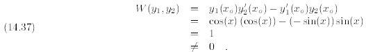
Since the Wronskian does not vanish, and must be linearly independent.