Singular Values

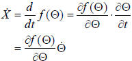
Usually with robots, we have a specification on the
velocity of the "end-effector" but we can only
measure the joint angles and their velocities. So to
determine the velocity of the tip of the robot, we take
the time-derivative:

	The Jacobian of the nonlinear transformation f.

In order to control the robot, we usually have a
specification, or desired velocity of the end
effector, The motor controllers, of course,
must receive angles (or angular velocities) as their
inputs, so given , we must compute the
necessary to achieve this , so that we can use it
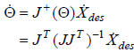
as a motor input. That is, we would like to solve
for

If J were square and nonsingular, we could simply use
the inverse of J. However, here J is 2 x 3:

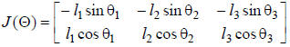
This is an example of a redundant system. There are an
infinite number of different combinations of joint angle
velocities that will give the same velocity . So that
the motors will go as slowly as possible, we often choose
the smallest one by employing the pseudoinverse:

NOTE: Recall that this is the "unweighted
pseudoinverse" that, in this case, will minimize

according to our earlier derivation.

In this situation, a "weighted" pseudoinverse is more
appropriate. If instead we do the derivation
minimizing the "weighted" norm

where B is a constant matrix, we will get a
pseudoinverse

The B-matrix can be used to "penalize" motion of the
heavier base-joint motors in favor of higher velocities
for the lighter wrist-joint motors; e.g.

Recall that the pseudoinverse can only be computed if
the J-matrix is of full rank, i.e., rank 2. If J is rank
deficient (this will depend on the angles ), we call
the configuration a singular configuration. One such
singular configuration is when all links are lined-up,
so the robot is extended into a straight-line. Singular
configurations represent a loss of a degree-offreedom
in the movement of the arm. For example,
when the arm is extended straight, it cannot
instantaneously move its tip inward or outward.

It is always good to keep the robot away from its
singular configurations. We can tell how close it is to
its singular configurations by examining the singular
values of the matrix J.

Obviously, if J is singular, then the product will
have a zero eigenvalue, so we can define a
"manipulability measure" as:

This is a nonnegative scalar-valued quantity that we
would like to keep away from zero.

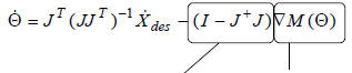
We can use the projection theorem to accomplish this in
our "inverse kinematics":

Suppose instead of using the regular pseudoinverse we
used:

orthogonal projection onto the null space of the Jacobian J.	gradient of the manipulability measure

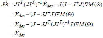
It is easy to show that adding this term to the previous
solution does not change the desired velocity of the
end effector by multiplying both sides by J:

So what does it do for us?

It contributes a component along the negative gradient of the
negative manipulability. Following the gradient of a
function tends to decrease the function, so following the
gradient of the negative of this function (which is always
positive) will tend to increase M.

That is, this term will automatically force the robot arm away
from any singular configurations as it moves.

We can draw "manipulability ellipsoids" that show how
well a robot can produce a velocity in various
configurations. The ellipsoid has axis-lengths equal to
the singular values, and axis directions along the
"singular vectors" (the columns of the U-matrix).

		Singular configuration
Can produce velocities equally well in both directions			Can produce velocities better in one direction than in the other.

For a more statistical error analysis, we can consider the
measurement of the joint angles as resulting from noisy
sensors which introduce an error . So the
measured joint angle is

where is the true value of the angle. If we assume that
the error term is a random variable that has zero
mean, and is uncorrelated among the different joints,
then the covariance matrix of the measured joint angle
vector is:

The terms are the variances of the individual sensor
error signals. Large terms indicate high uncertainty
for those measurements.

Substituting the noisy sensor readings into the
kinematic equations:

Now if we assume the quantities are small, we can
linearize this equation by finding the first two terms
of the Talyor series expansion, which gives:

where

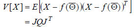
The expected value of X is now

while the covariance of X is:

If we now find the singular value decomposition of this
matrix, we can use the information to draw
"uncertainty ellipsoids":

Once again, the columns of U are vectors that give the
directions of the axes of the ellipsoid, and the singular
values tell us the lengths of those axes.

Intuitively, we have drawn an ellipsoid that indicates
our uncertainty in the measurement of the end
effector location in different directions.

If a sensor in one particular joint is very noisy, then the
corresponding term in Q will be large, and the
corresponding axis length will be large. This
translates to a large uncertainty in a particular
coordinate of the location of the end effector.

For more information:

Klema, V. C., and A. J. Laub, "The Singular Value
Decomposition: Its Computation and Some
Applications," IEEE Trans. Auto. Control, vol. AC-25,
no. 2, April 1980, pp. 164-176.

Press, W. H. et al, Numerical Recipes in C: The Art of
Scientific Computing, Cambridge: Cambridge
University Press, 1988, pp. 60-72.